Analyzing the Netflix Catalog

In this post, we're going to explore the Netflix catalog using a dataset available on Kaggle. This analysis will allow us to better understand the patterns and trends of the films and series available on the platform. This post integrates fundamental concepts of data analysis, data collection and cleaning, exploratory analysis and statistical modeling that we have discussed previously on the blog.

Throughout our data analysis journey, we have learned the importance of understanding the context and purpose of our study. The Netflix dataset is an excellent opportunity for us to apply our skills and discover valuable insights into the content available on the platform.

For this analysis, we will apply concepts such as data exploration, visualization and statistical modeling. We will use popular Python libraries such as pandas, matplotlib, seaborn and scikit-learn.

Database

Before we dive into the analysis, it's important to understand the database we'll be using. We'll be working with the Netflix dataset available on Kaggle, which comprises a detailed catalog of films and series available on the platform until mid-2021. This dataset is a tabular database, containing 8,809 entries and 12 columns, each representing different aspects of the titles.

The columns we will use in our analysis are:

• show_id: A unique identifier for each title.

• type: The category of the title, which can be 'Movie' or 'TV Show'.

• title: The name of the movie or series.

• director: The director(s) of the title. This column may contain null values for some entries, especially series.

• cast: The list of main actors in the title. This column can also have null values.

• country: The country(ies) where the movie or series was produced.

• date_added: The date the title was added to Netflix.

• release_year: The year in which the movie or series was originally released.

• rating: The age rating of the title.

• duration: The length of the title, in minutes for movies and in seasons for series.
  

• listed_in: The genres to which the title belongs.

• description: A brief summary of the title.

We will use this data to carry out a detailed analysis of the Netflix catalog, exploring patterns and trends in the content available.

Tools used:

• Pandas: for data manipulation and analysis.

• Matplotlib and Seaborn for data visualization.

• Scikit-learn for statistical analysis and predictive modeling.

Libraries used

import pandas as pd
import matplotlib.pyplot as plt
import seaborn as sns

from sklearn.model_selection import train_test_split
from sklearn.linear_model import LogisticRegression
from sklearn.metrics import classification_report

Data collection and cleaning

First, we'll import the dataset and do some initial cleaning. We'll check for missing data and deal with inconsistencies.

# Loading the dataset
url = 'netflix_titles.csv'
df = pd.read_csv(url)

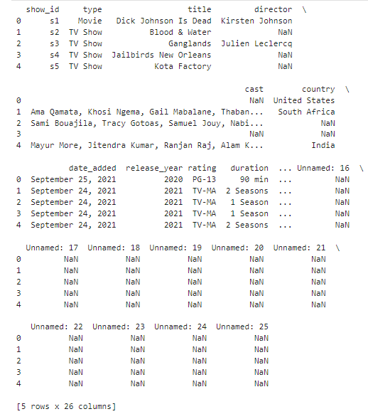
# Viewing the firt lines of the dataset
print(df.head())

# Checking for missing data
print(df.isnull().sum())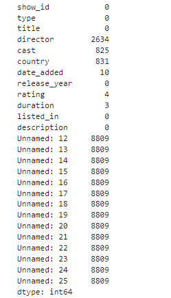

# Filling in missing values
df['director'].fillna('Unknown', inplace=True)
df['cast'].fillna('Unknown', inplace=True)
df.dropna(subset=['country', 'date_added', 'rating'], inplace=True)

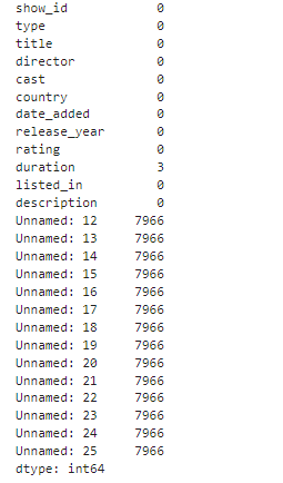
# Confirming that there are no more missing values
print(df.isnull().sum())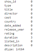

# Removing unnamed columns
df.dropna(axis=1, how='all', inplace=True)
# Confirming that there are no more missing values
print(df.isnull().sum())

Exploring the Data Analysis Area

Now that our data is clean, we can explore different aspects of the Netflix catalog. Let's start by analyzing the distribution of films and series over the years.

# Distribution of films and series over the years
plt.figure(figsize=(12,6))
sns.histplot(df['release_year'], bins=30, kde=True)
plt.title('Distribution of films and series by year of release')
plt.xlabel('Release Year')
plt.ylabel('Count')
plt.show()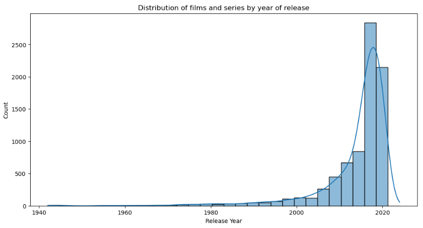

Exploratory Analysis

Let's deepen our exploratory analysis by examining the popularity of genres over time and the geographical distribution of productions.

# Separating the genres into individual lines
df_genres=df['listed_in'].str.split(',', expand=True).stack().reset_index(level=1, drop=True)
df_genres.name = 'genre'
df_genres = df_genres.to_frame()

# Counting the frequency of each genre
genre_counts = df_genres['genre'].value_counts()

# Keeping only the 10 most popular genres
top_10_genres = genre_counts.head(10)

# Visualizing the 10 most popular genres
plt.figure(figsize=(12,6))
bar_plot = sns.barplot(y=top_10_genres.index, x=top_10_genres.values, palette='viridis', dodge=False)
plt.title('Top 10 Most Popular Genres')
plt.xlabel('Count')
plt.ylabel('Genre')

# Adding the count to the end of each bar
for index, value in enumerate(top_10_genres.values):
    plt.text(value, index, str(value), va='center')

plt.show()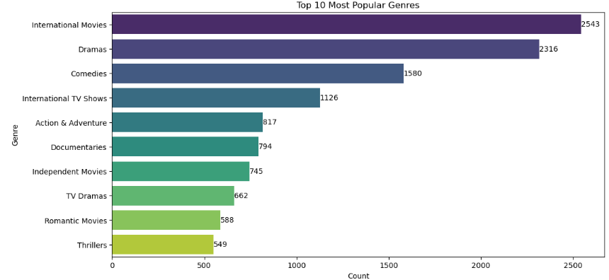

# Counting the frequency of productions by country
country_counts = df['country'].value_counts()

# Keeping only the 10 countries with the most productions
top_10_countries = country_counts.head(10)

# Visualizing the 10 countries with the most productions
plt.figure(figsize=(12, 6))
sns.barplot(y=top_10_countries.index,x=top_10_countries.values,palette='viridis', dodge=False)
plt.title('Top 10 Countries with the Most Productions on Netflix')
plt.xlabel('Countries')
plt.ylabel('Country')
plt.show()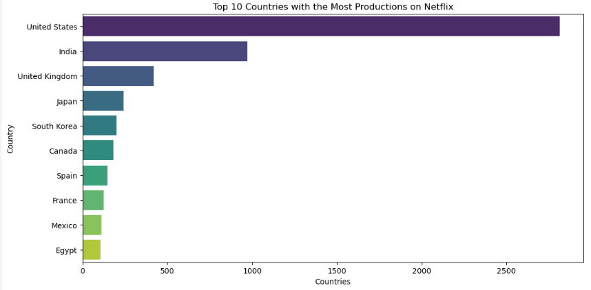

# Trends in the average length of films: an analysis over the years
# Filling in missing values
df['director'].fillna('Unknown', inplace=True)
df['cast'].fillna('Unknown', inplace=True)
df.dropna(subset=['country', 'date_added', 'rating'], inplace=True)
def convert_seasons_to_minutes(duration):
    if isinstance(duration, str) and 'Season' in duration: # Extract the number of seasons
        seasons = int(duration.split(' ')[0])

        # Convert seasons to minutes (assuming a season has an average of 10 episodes and each episode has an average of 30 minutes)
        return seasons * 10 * 30
    elif isinstance(duration, float):
        # If the value is a float (possibly NaN), return NaN
        return duration
    else:
        # If the value is not a 'Season' string, it is assumed to be a number of minutes already
        return int(duration.split(' ')[0])

# Converting the 'duration' column to minutes format
df['duration']=df['duration'].apply(convert_seasons_to_minutes)# Removing extra spaces before and after the values in the 'date_added' column
df['date_added'] = df['date_added'].str.strip()
# Converting the 'date_added' column to the datetime type
df['date_added'] = pd.to_datetime(df['date_added'], errors='coerce')
# Extracting the release year
df['release_year'] =pd.DatetimeIndex(df['date_added']).year

# Calculating the average duration over the years
mean_duration_year = df.groupby('release_year')['duration'].mean()

# Visualizing the average duration over the years
plt.figure(figsize=(12, 6))
line_plot_duration = mean_duration_year.plot(kind='line', marker='o', color='b')
plt.title('Average Duration Over Years')
plt.xlabel('Release Year')
plt.ylabel('Average Duration (minutes)')
plt.grid(True)

# Adding the average duration to the end of each point in the line graph
for year, duration in mean_duration_year.items(): plt.text(year, duration, f'{duration:.2f}', ha='center', va='bottom')

plt.show()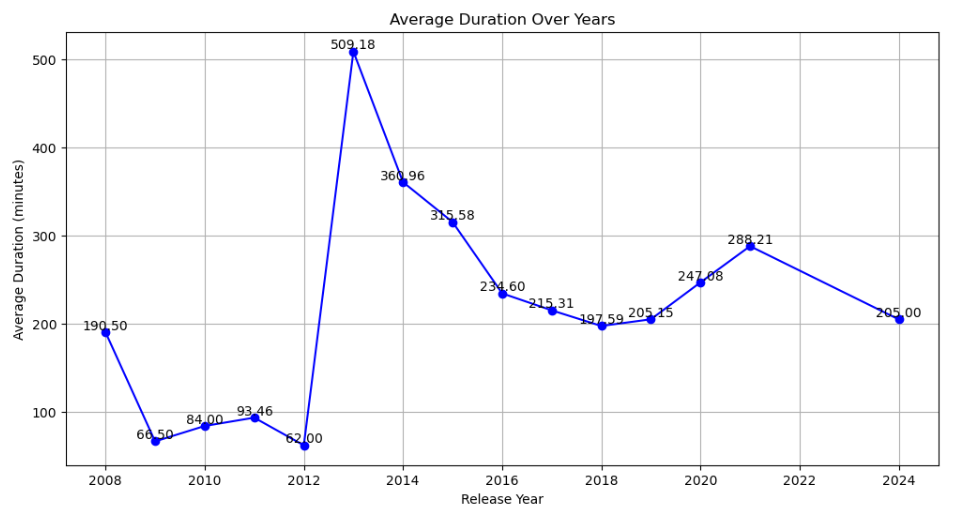

Basic statistical modeling

To better understand the correlations between different variables, we can apply basic statistical modeling techniques.

# Selecting only the movies and creating a copy to avoid modifying the original DataFrame
df_movies = df[df['type'] == 'Movie'].copy()

# Removing the ' min' suffix from the duration column and converting to integer
df_movies['duration'] = df_movies['duration'].apply(lambda x: int(x.split(' ')[0]) if isinstance(x, str) else x)

# Dealing with missing values in the duration column
df_movies.dropna(subset=['duration'], inplace=True)

# Creating a linear regression model
model = LinearRegression()

# Separating the independent (X) and dependent (y) variables
X = df_movies['release_year'].values.reshape(-1, 1) # Year of release
y = df_movies['duration'].values.reshape(-1, 1) # Duration of films

# Dealing with missing values in the dependent variable (y)
y = np.nan_to_num(y)

# Training the model
model.fit(X, y)

# Predicting the length of movies based on the year of release
y_pred = model.predict(X)

# Plotting the relationship between duration and year of release with the regression line
plt.figure(figsize=(12,6))
sns.scatterplot(x='release_year',y='duration',data=df_movies)
plt.title('Duration of films over the years')
plt.xlabel('Release Year')
plt.ylabel('Duration (minutes)')
plt.show()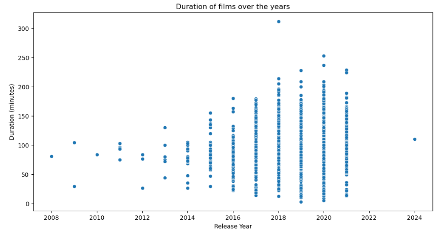

Predictive Statistical Modeling

Finally, we can build a simple predictive model to predict the popularity of genres based on the characteristics of the titles.

# Data preparation
df['label'] = df['listed_in'].apply(lambda x: 1 if 'Dramas' in x else 0)
X = df[['release_year', 'duration']].dropna()
y = df['label'].dropna()

# Splitting the data into training and test
X_train, X_test, y_train, y_test = train_test_split(X, y, test_size=0.3, random_state=42)

# Traininmodel
model = LogisticRegression(class_weight='balanced')
model.fit(X_train, y_train)

# Evaluating the model
y_pred = model.predict(X_test)
print(classification_report(y_test, y_pred))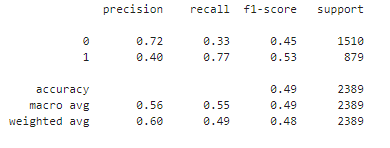

The data model shows that it gets it right about 72% of the time when predicting whether a genre is popular or not. However, it struggles to correctly detect popular genres, getting only 33% of them right. For less popular genres, it is more successful, getting about 77% of them right, but still with some errors. We need to adjust the model so that it can make more balanced and reliable predictions.

Conclusion

In this article, we carry out a detailed analysis of the Netflix catalogue using a dataset available on Kaggle. We explore various facets of the platform's films and series, applying concepts of data analysis, cleaning and manipulation, visualisation and statistical modelling.

We started by importing and cleaning the dataset, dealing with missing values and inconsistencies. We used the pandas library for data manipulation, checking the integrity of the set before moving on to exploratory analysis. An initial check revealed null values in the director, cast, country, date added and age rating columns. We filled in missing values for director and cast with ‘Unknown’ and removed entries with missing values in the other columns mentioned.

In the exploratory analysis, we examined the temporal distribution of film and series releases, identifying interesting patterns over the years. We visualised the popularity of genres, where the 10 most popular were highlighted, and analysed the geographical distribution of productions, identifying the top 10 countries of origin. This analysis revealed a predominance of certain genres and countries, offering a clear view of the preferences and trends of the content available on Netflix.

To analyse the length of films over the years, we converted the length of series into minutes. We observed a slight upward trend in the average length of films over time. This analysis was visualised in a line graph, where each point represented the average length of the films per year of release.

In terms of statistical modelling, we applied a linear regression to investigate the relationship between the length of films and the year of release. This modelling helped confirm the trend observed in the exploratory analysis. Although the relationship between these variables was not very strong, the linear regression served as a good introduction to the application of modelling techniques in our study.

For a predictive analysis, we built a logistic regression model to predict the popularity of the genres based on the characteristics of the titles. We split the data into training and test sets, using the release year and duration columns as independent variables. The model achieved an overall accuracy of 72 per cent, but struggled to correctly detect popular genres, highlighting the need for adjustments and refinements. This result showed us the complexity of predicting genre popularity and the importance of exploring additional variables and more advanced techniques to improve accuracy.

In summary, the analysis of the Netflix catalogue provided us with valuable insights into the patterns and trends of the content available on the platform. However, we identified areas for improvement, especially in predictive modelling. Future analyses could benefit from the inclusion of more explanatory variables and the use of advanced machine learning techniques. This analysis reinforces the importance of data cleaning and careful choice of analytical techniques in order to obtain meaningful results. I hope this study has been enlightening and useful for readers interested in data analysis. Keep following the blog for more analyses and insights in future articles.